CPU vs GPU

Every number on this page comes from one run of benchmarks/run_benchmarks.sh on a single machine:

CPU	AMD Ryzen 9 3950X 16-Core Processor (32 logical cores, torch using 16 threads)
GPU 0	NVIDIA GeForce RTX 3090
GPU 1	NVIDIA GeForce RTX 3080
PyTorch	2.10.0+cu128 / CUDA 12.8
torchtsetlin	0.6.0
Python	3.10.11
measured	2026-10-29 09:10:06

How to read these

Each point is the median of three timed blocks of steady-state calls, after a warm-up, with the device synchronised once per block. The micro-benchmarks use synthetic Boolean data at 20 % density, resident on the device unless stated otherwise. Reproduce — or replace these numbers with your own hardware's — with:

./benchmarks/run_benchmarks.sh          # ~20-25 min, rewrites this page

These are the numbers of torchtsetlin 0.6.0. Benchmark history puts the same suites side by side for every earlier version.

Throughput vs batch size

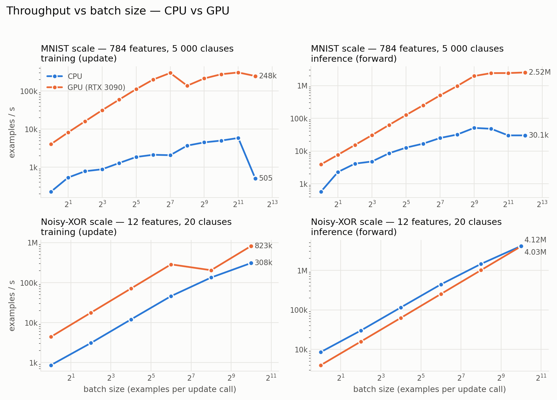
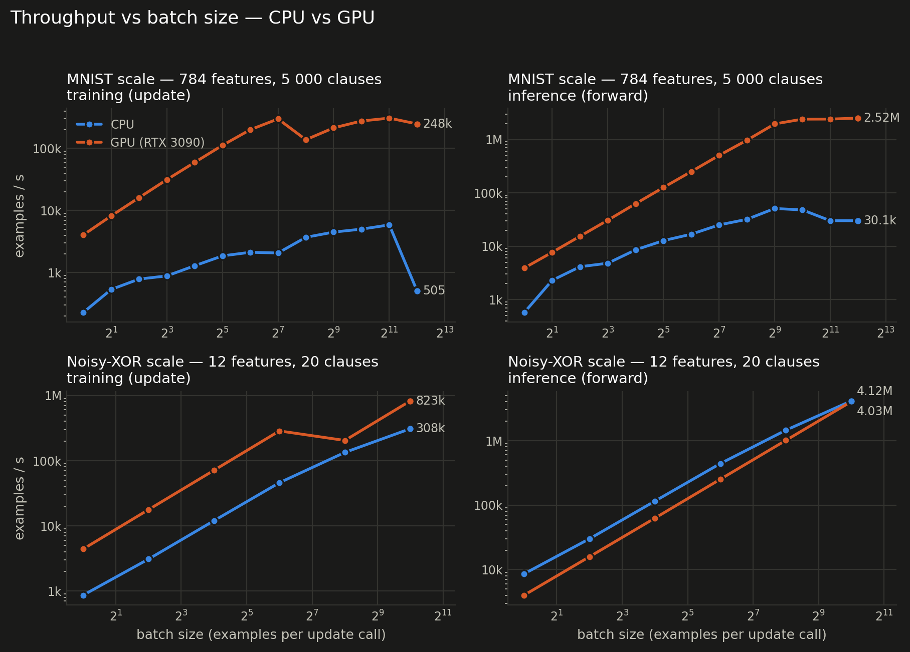
One update() call touches every automaton in the machine, so its cost depends far more on the size of the machine than on how many examples are in the batch. Feeding the GPU more examples per call is therefore nearly free: training throughput rises from 4,042 examples/s at batch 1 to 248,421 at batch 4096. At batch 256 the same model trains 138,358 examples/s on the GPU against 3,692 on the CPU (37×).

The Noisy-XOR scale machine in the bottom row is the counter-example: 20 clauses over 12 features is less work than a kernel launch, so only past batch 1 does the GPU pull ahead. Small machines belong on the CPU.

Batch size — MNIST scale (784 features, 500 clauses/class)

batch	CPU train ex/s	GPU train ex/s	train speedup	CPU infer ex/s	GPU infer ex/s	infer speedup
1	228	4,042	17.8×	574	3,906	6.8×
2	533	8,187	15.4×	2,290	7,680	3.4×
4	783	16,086	20.5×	4,118	15,358	3.7×
8	881	31,405	35.6×	4,793	30,683	6.4×
16	1,285	59,537	46.3×	8,536	62,631	7.3×
32	1,853	112,278	60.6×	12,708	126,117	9.9×
64	2,119	200,553	94.6×	16,779	250,169	14.9×
128	2,065	299,217	144.9×	25,023	502,813	20.1×
256	3,692	138,358	37.5×	31,858	968,265	30.4×
512	4,487	214,686	47.8×	50,911	1,958,782	38.5×
1,024	5,000	277,166	55.4×	47,860	2,410,515	50.4×
2,048	5,854	308,585	52.7×	30,055	2,417,111	80.4×
4,096	505	248,421	491.9×	30,085	2,520,419	83.8×

Batch size — Noisy-XOR scale (12 features, 10 clauses/class)

batch	CPU train ex/s	GPU train ex/s	train speedup	CPU infer ex/s	GPU infer ex/s	infer speedup
1	864	4,403	5.1×	8,572	3,998	0.5×
4	3,090	17,714	5.7×	29,995	15,801	0.5×
16	11,979	71,039	5.9×	115,284	62,742	0.5×
64	45,845	285,206	6.2×	440,671	251,805	0.6×
256	133,553	203,689	1.5×	1,448,447	1,007,928	0.7×
1,024	308,262	822,790	2.7×	4,124,239	4,026,418	1.0×

How much the GPU buys you

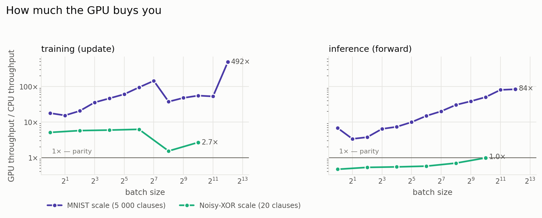
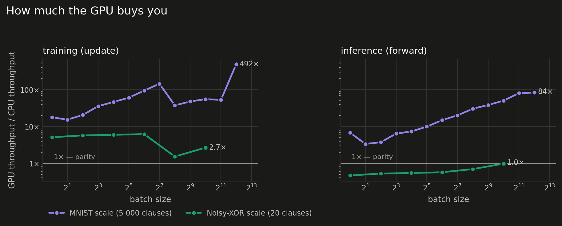
The speedup is not one number. It grows with batch size because the CPU pays the per-clause cost serially while the GPU hides it, peaks at about 492× around batch 4096, and holds from there. Inference behaves differently again: the CPU forward pass is already cheap, so the gap there tops out at 84× — worth having, but not the same kind of difference.

Throughput vs model size

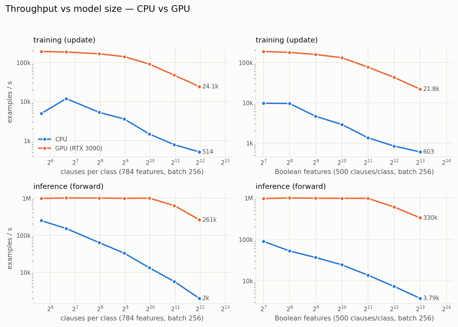
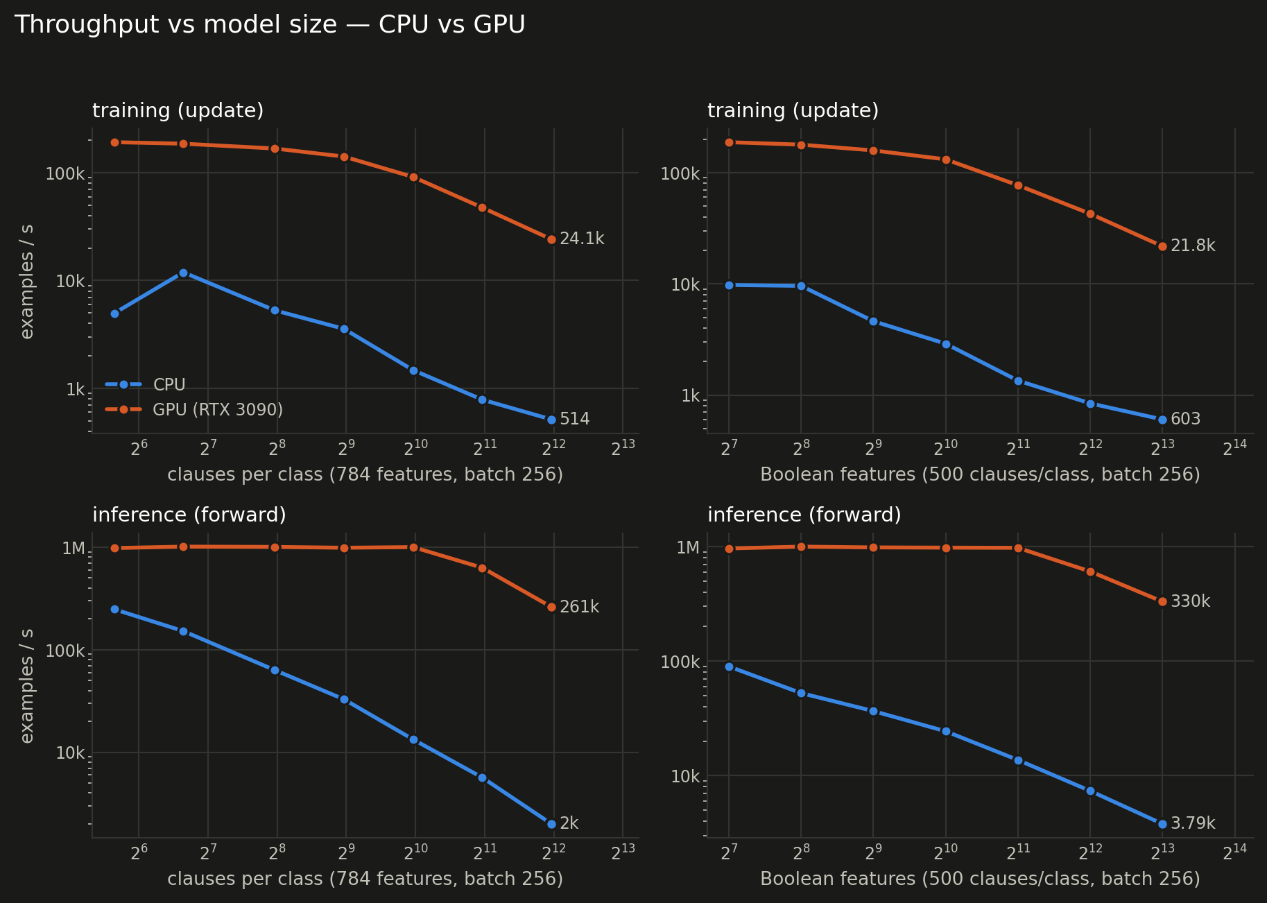
Both axes cost the same thing — the update is n_clauses × 2 × n_features element-wise work — so both curves fall roughly as 1/x. The CPU falls off immediately; the GPU stays flat until the machine is big enough to fill it, which is why the gap widens with model size: 39× at 50 clauses/class against 47× at 4000; 19× at 128 features against 36× at 8192. Big machines are exactly the ones worth moving to a GPU.

Clause budget (784 features, batch 256)

clauses/class	CPU train ex/s	GPU train ex/s	train speedup	CPU infer ex/s	GPU infer ex/s	infer speedup
50	4,961	192,140	38.7×	248,098	979,219	3.9×
100	11,918	186,057	15.6×	151,742	1,011,026	6.7×
250	5,290	167,860	31.7×	63,210	1,004,436	15.9×
500	3,560	141,289	39.7×	32,815	985,867	30.0×
1,000	1,474	91,372	62.0×	13,330	1,000,287	75.0×
2,000	784	47,474	60.6×	5,661	629,095	111.1×
4,000	514	24,116	46.9×	1,999	260,728	130.4×

Feature count (500 clauses/class, batch 256)

features	CPU train ex/s	GPU train ex/s	train speedup	CPU infer ex/s	GPU infer ex/s	infer speedup
128	9,768	187,734	19.2×	89,701	960,951	10.7×
256	9,587	178,397	18.6×	52,506	997,185	19.0×
512	4,613	158,266	34.3×	36,591	981,522	26.8×
1,024	2,897	131,572	45.4×	24,392	977,050	40.1×
2,048	1,349	77,025	57.1×	13,695	973,727	71.1×
4,096	842	42,651	50.6×	7,355	605,203	82.3×
8,192	603	21,766	36.1×	3,787	330,395	87.2×

The model zoo

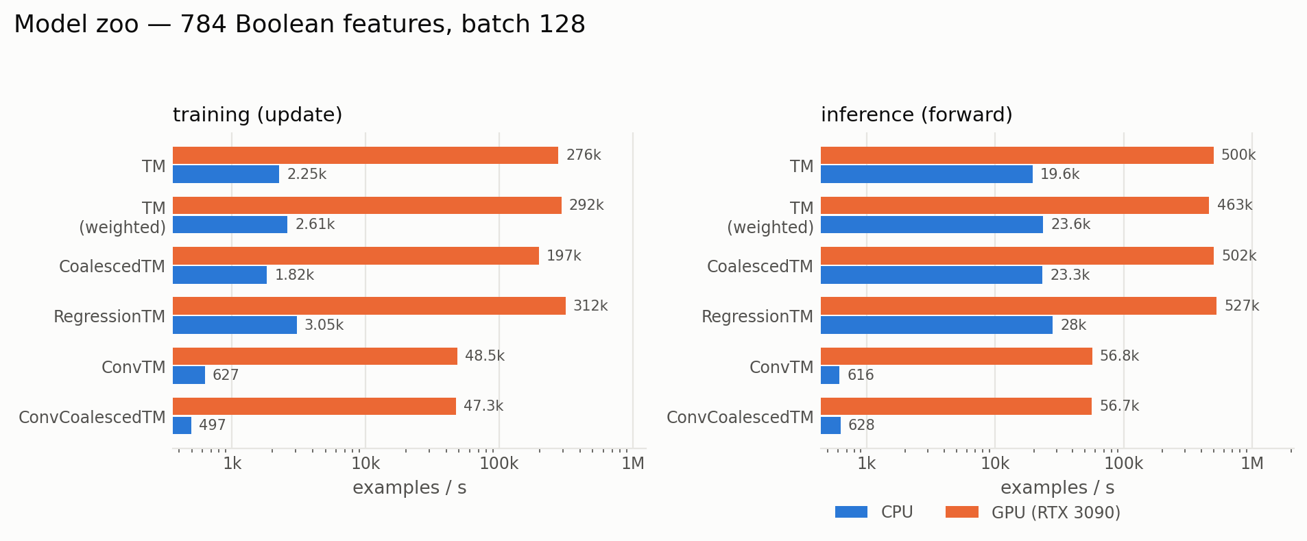
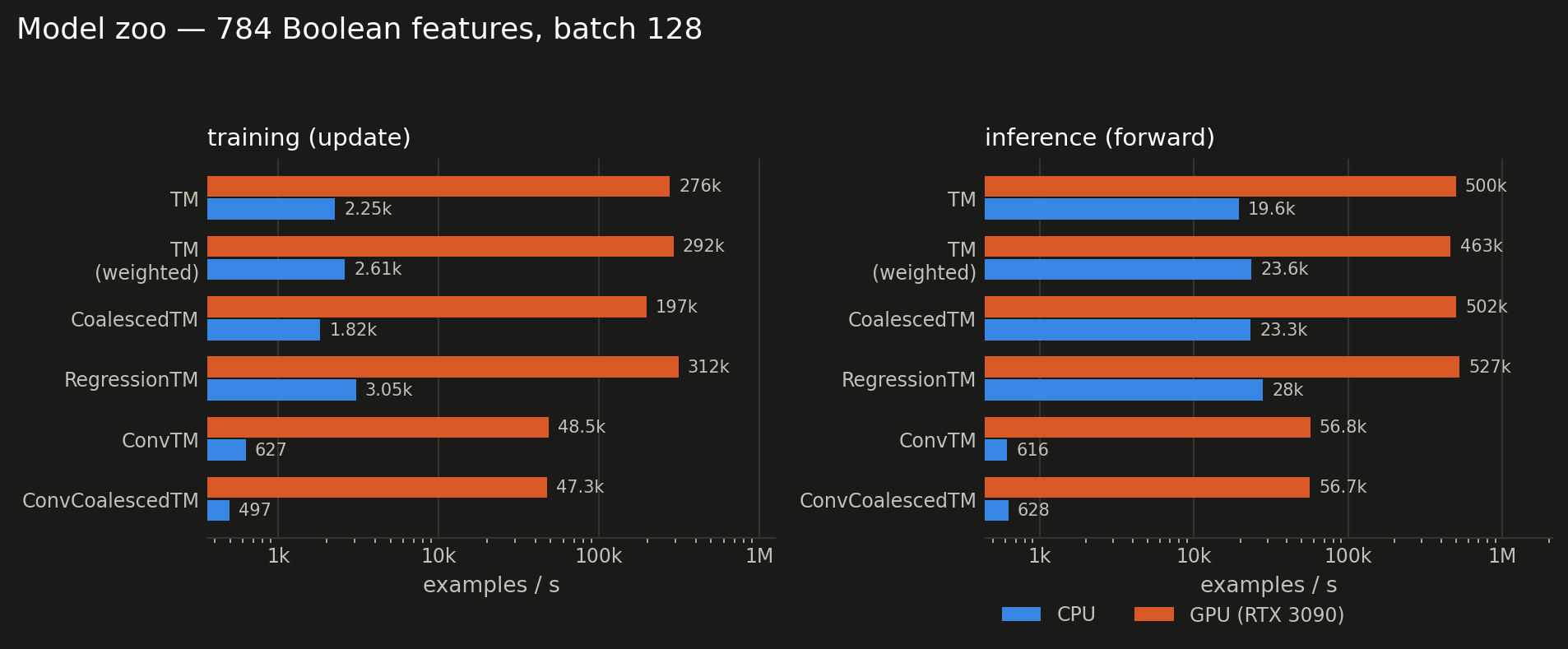
Weighted and coalesced variants cost about what the plain machine costs: they change the output layer and the feedback policy, not the per-clause work that dominates. The convolutional models are the outlier at 6× the cost of the flat machine per example — a 10×10 patch over a 28×28 image is 361 patches, and every patch is evaluated against every clause.

Model zoo (784 features, batch 128)

model	CPU train ex/s	GPU train ex/s	train speedup	CPU infer ex/s	GPU infer ex/s	infer speedup	GPU peak memory
TsetlinMachine	2,251	275,696	122×	19,614	500,053	25×	55 MB
TsetlinMachine (weighted)	2,608	292,007	112×	23,596	462,666	20×	56 MB
CoalescedTsetlinMachine	1,823	197,189	108×	23,299	501,733	22×	64 MB
RegressionTsetlinMachine	3,047	312,436	103×	27,998	527,448	19×	56 MB
ConvTsetlinMachine	627	48,537	77×	616	56,769	92×	167 MB
ConvCoalescedTsetlinMachine	497	47,276	95×	628	56,652	90×	167 MB

Where an update goes

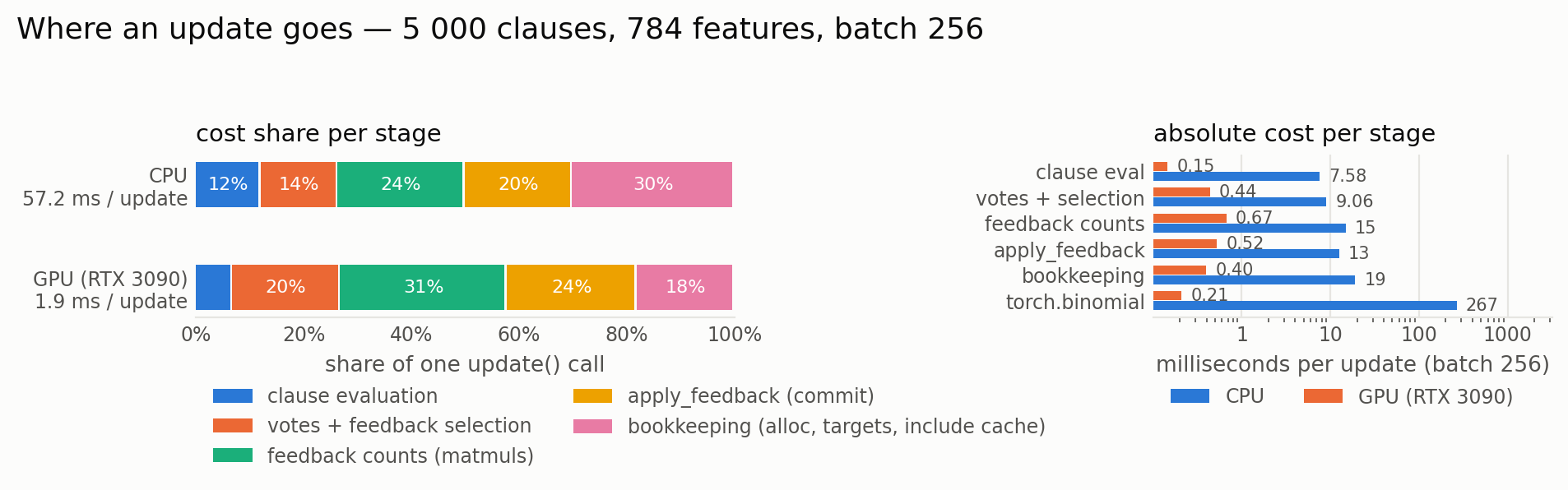
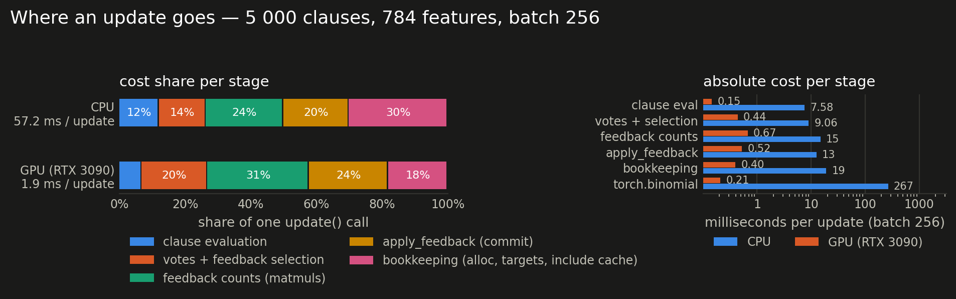
apply_feedback — the stochastic increment/decrement of the whole (n_clauses, 2F) automaton state — is the expensive part of an update: on the CPU it is 22 % of the 57.2 ms call; on the GPU it is 28 % of the 1.9 ms call. A standalone torch.binomial draw of the same (C, 2F) shape costs 266.65 ms on the CPU and 0.21 ms on the GPU — the single most expensive op in the commit. Everything before the commit (encoding, clause evaluation, the vote sums and the feedback count matmuls) is comparatively cheap. That is also why batching pays: a batched update draws once per commit, a sequential one draws once per example.

Update cost breakdown (5 000 clauses, 784 features, batch 256)

stage	cpu (ms)	cuda:0 (ms)
encode	0.075	0.038
evaluate	7.508	0.108
votes+select	9.059	0.436
feedback_counts	14.962	0.675
accumulator_alloc	3.800	0.117
coerce_targets	0.009	0.052
apply_feedback	12.591	0.525
refresh_include	15.303	0.227
commit	27.903	0.803
torch.binomial (C x 2F)	266.648	0.209
update() total	57.181	1.876

CPU thread scaling

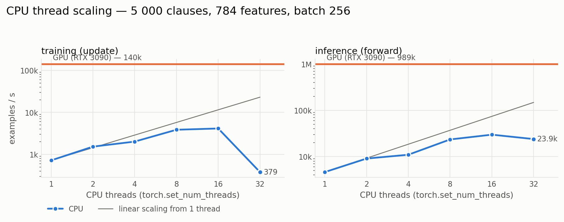
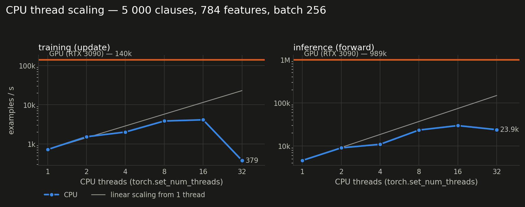
More CPU threads buy surprisingly little in training: 0.5× going from 1 to 32 threads. The batched update is a chain of large element-wise ops over the state, and the binomial draw that dominates it does not thread. Inference scales much better (5.2× over the same range): the forward pass is one big matmul-shaped reduction. If a CPU run is too slow, the lever is the clause budget or the batch size, not torch.set_num_threads.

CPU thread scaling (5 000 clauses, 784 features, batch 256)

threads	train ex/s	infer ex/s
1	720	4,629
2	1,528	9,072
4	2,015	10,974
8	3,860	23,464
16	4,136	29,778
32	379	23,923

Batched vs sequential feedback

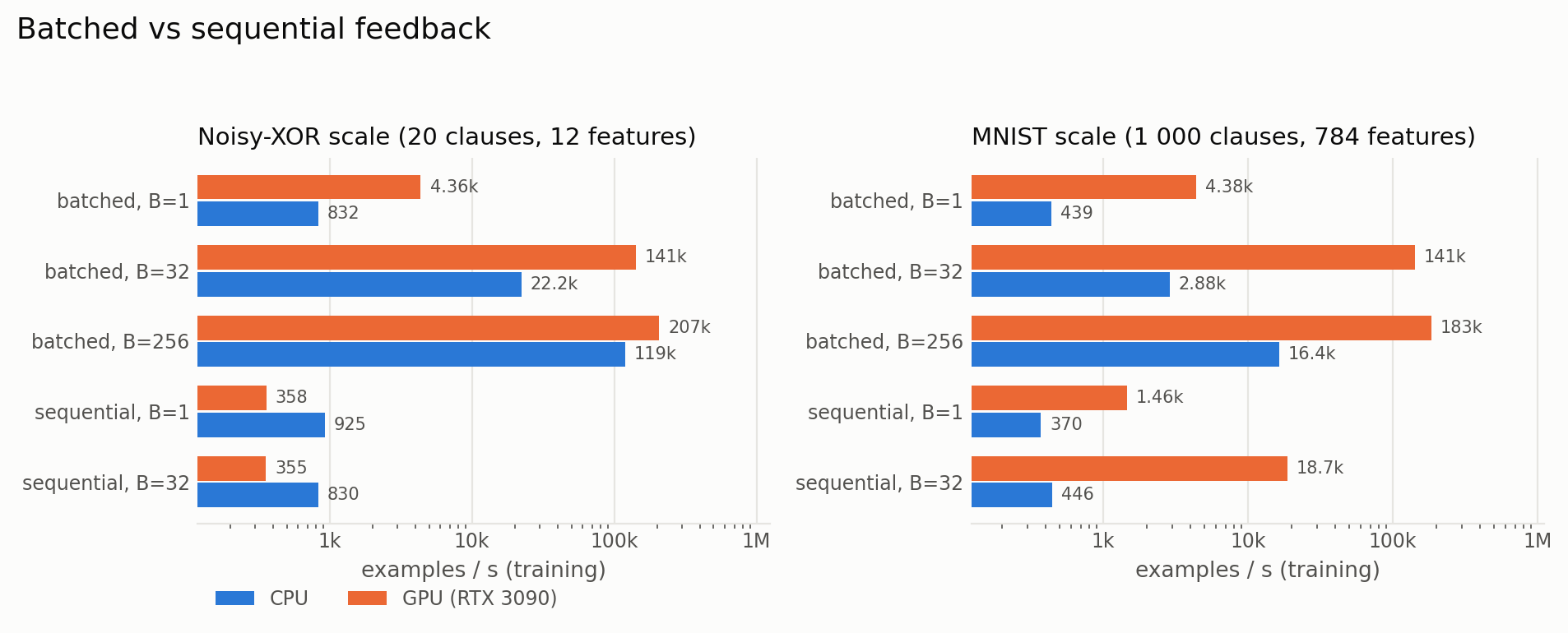
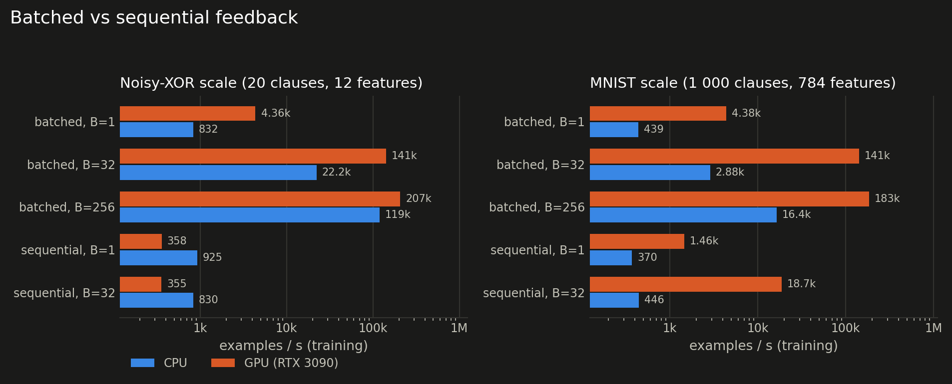
feedback_mode="sequential" is the exact per-example algorithm: it commits once per example, so a mini-batch of 32 pays 32 commits instead of one. Measured at batch 32 that is 6-399× slower than the batched update, depending on the model scale and the device. Batching is the default for that reason — but it is an approximation, and its fidelity degrades as the batch grows. See Batched vs sequential feedback for the accuracy side of this trade.

Batched vs sequential feedback

scale	feedback_mode	batch	device	examples/s	ms / update call
mnist-1k	batch	1	cpu	439	2.28
mnist-1k	batch	1	cuda:0	4,377	0.23
mnist-1k	batch	32	cpu	2,878	11.12
mnist-1k	batch	32	cuda:0	141,337	0.23
mnist-1k	batch	256	cpu	16,428	15.58
mnist-1k	batch	256	cuda:0	183,495	1.40
mnist-1k	sequential	1	cpu	370	2.70
mnist-1k	sequential	1	cuda:0	1,456	0.69
mnist-1k	sequential	32	cpu	446	71.72
mnist-1k	sequential	32	cuda:0	18,667	1.71
xor	batch	1	cpu	832	1.20
xor	batch	1	cuda:0	4,364	0.23
xor	batch	32	cpu	22,225	1.44
xor	batch	32	cuda:0	141,475	0.23
xor	batch	256	cpu	119,070	2.15
xor	batch	256	cuda:0	207,292	1.23
xor	sequential	1	cpu	925	1.08
xor	sequential	1	cuda:0	358	2.79
xor	sequential	32	cpu	830	38.57
xor	sequential	32	cuda:0	355	90.20

Where the data lives

Keeping the Boolean dataset in host memory and copying each mini-batch across costs at most 4 % of throughput here — the update is long enough to hide the transfer. So stream a dataset that does not fit in VRAM without worrying, but do hand the model a device tensor: see Choosing a device for the one copy that does bite (Booleanization encoders keep their thresholds on the CPU).

Host- vs device-resident data (training, 784 features, 500 clauses/class)

device	batch	dataset lives on	examples/s	ms / update
cpu	32	device	1,420	22.54
cpu	32	host	1,366	23.43
cpu	256	device	3,538	72.36
cpu	256	host	3,570	71.70
cpu	2048	device	5,268	388.80
cpu	2048	host	5,719	358.10
cuda:0	32	device	101,124	0.32
cuda:0	32	host	104,502	0.31
cuda:0	256	device	136,039	1.88
cuda:0	256	host	135,599	1.89
cuda:0	2048	device	305,019	6.71
cuda:0	2048	host	301,221	6.80

Dense segmentation

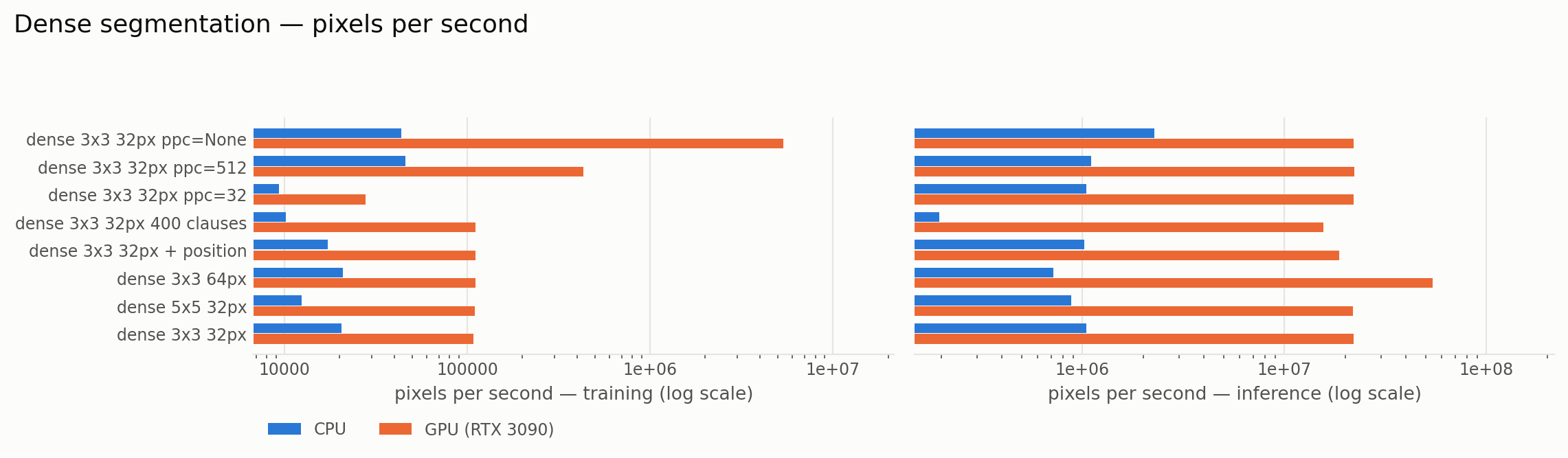
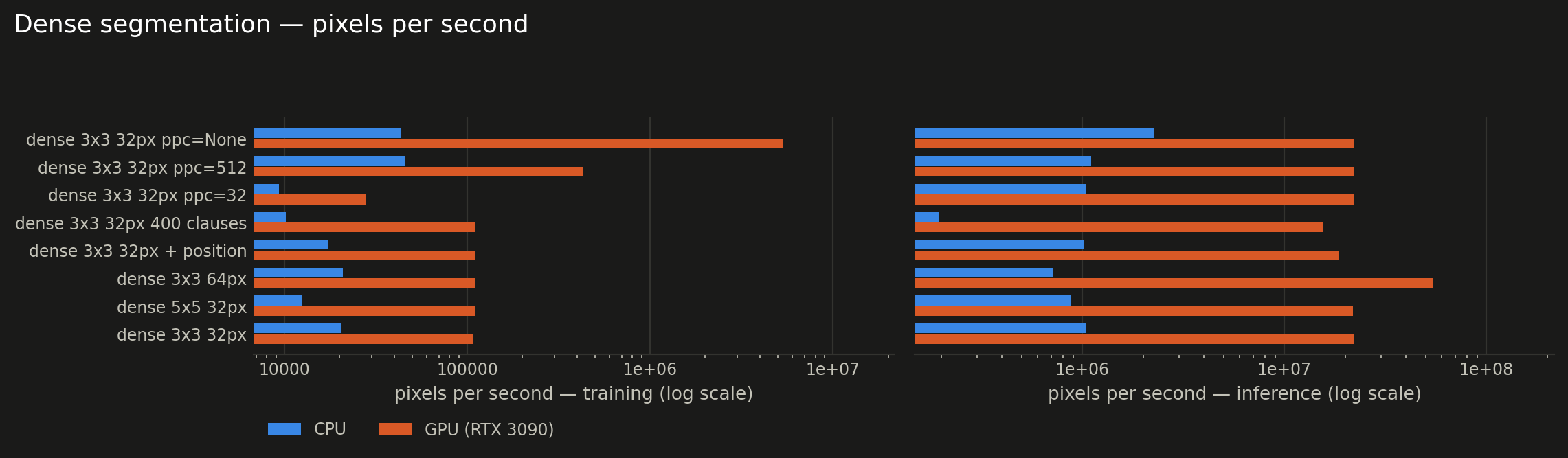
Dense prediction evaluates one patch per pixel, so throughput is quoted in pixels per second rather than examples per second — one 32×32 image is 1 024 examples.

• A 3×3 dense model on 32×32 inputs runs at 20,472 px/s training and 1,048,820 px/s predicting on CPU — prediction is roughly 51× cheaper, because it never draws feedback or touches the automata.
• patches_per_commit is the price of fidelity: committing once per batch reaches 43,432 px/s against 20,472 at the default 128, a 2.1× speedup that costs real accuracy (see the segmentation guide's ablation).

Dense segmentation (4 planes, 4 classes, batch 8 images)

configuration	patches/commit	CPU train px/s	GPU train px/s	train speedup	CPU infer px/s	GPU infer px/s	infer speedup
dense 3x3 32px	128	20,472	107,750	5×	1,048,820	21,982,433	21×
dense 5x5 32px	128	12,402	109,839	9×	876,901	21,861,851	25×
dense 3x3 64px	128	20,813	111,119	5×	716,707	54,257,194	76×
dense 3x3 32px + position	128	17,291	111,121	6×	1,022,430	18,601,999	18×
dense 3x3 32px 400 clauses	128	10,172	111,073	11×	195,079	15,617,485	80×
dense 3x3 32px ppc=32	32	9,329	27,881	3×	1,047,587	21,967,614	21×
dense 3x3 32px ppc=512	512	45,850	429,667	9×	1,107,562	22,158,173	20×
dense 3x3 32px ppc=None	all	43,432	5,368,704	124×	2,277,724	21,918,503	10×

3D convolution

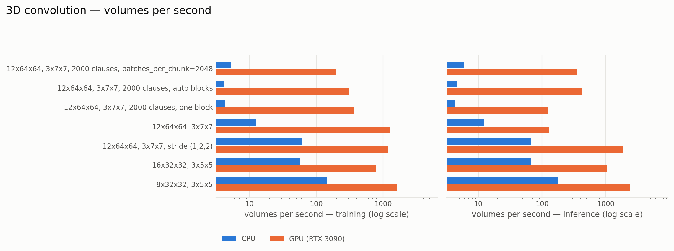
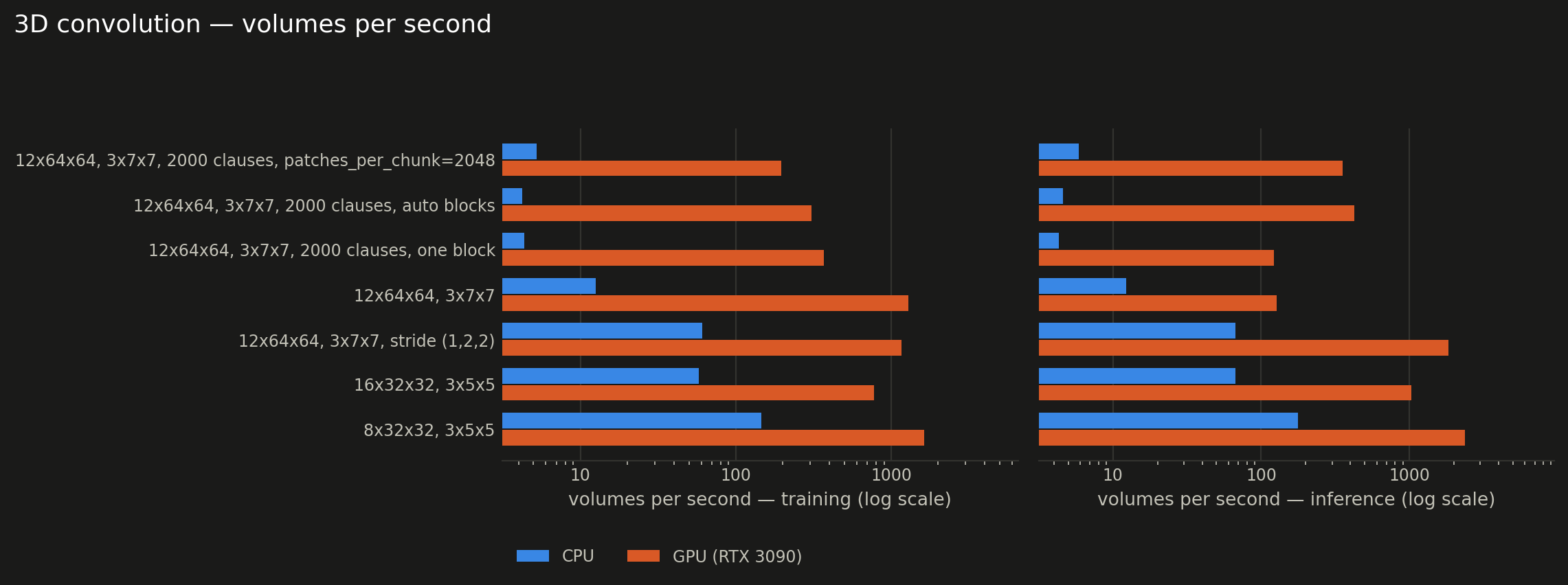
A 3D convolutional machine evaluates every clause at every window position of a volume, so the cost scales with the number of positions P = Pd·Ph·Pw. Throughput is quoted in volumes per second.

• On GPU (RTX 3090), a cardiac-sized 12×64×64 volume with a 3×7×7 window has 33,640 window positions and trains at 1,287.2 volumes/s; an in-plane stride of 2 cuts that to 8,410 positions and runs at 1,168.8 volumes/s (0.9×).
• With 2 000 clauses one such volume no longer fits max_chunk_elements, so the patch axis is split automatically into blocks of 18,982 positions: peak memory 247 MB at 306.05 volumes/s, against 268 MB at 367.61 volumes/s when it is forced into one block. The output is identical (the OR over patches and the random-patch draw are exact under the split); with fewer clauses, ordinary batch chunking already respects the budget and blocking buys nothing.

3D convolution (1 plane; 2 x 100 clauses, batch 4 — or 10 x 200, batch 2)

configuration	patches P	patches per block	CPU train vol/s	GPU train vol/s	train speedup	CPU infer vol/s	GPU infer vol/s	infer speedup	GPU peak memory (train)
8x32x32, 3x5x5	4,704	4,704	146.6	1,633.1	11×	176.5	2,372.2	13×	60 MB
16x32x32, 3x5x5	10,976	10,976	57.6	776.7	13×	66.8	1,027.1	15×	142 MB
12x64x64, 3x7x7, stride (1,2,2)	8,410	8,410	60.8	1,168.8	19×	67.2	1,832.5	27×	170 MB
12x64x64, 3x7x7	33,640	33,640	12.6	1,287.2	102×	12.3	127.5	10×	360 MB
12x64x64, 3x7x7, 2000 clauses, one block	33,640	33,640	4.4	367.6	84×	4.3	121.8	28×	268 MB
12x64x64, 3x7x7, 2000 clauses, auto blocks	33,640	18,982	4.2	306.0	72×	4.6	426.3	92×	247 MB
12x64x64, 3x7x7, 2000 clauses, patches_per_chunk=2048	33,640	2,048	5.2	195.8	37×	5.9	352.8	60×	266 MB

End to end: MNIST

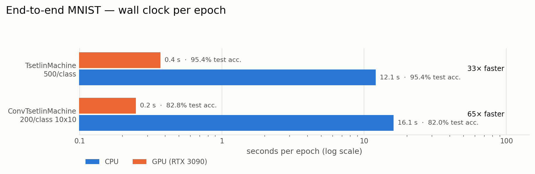
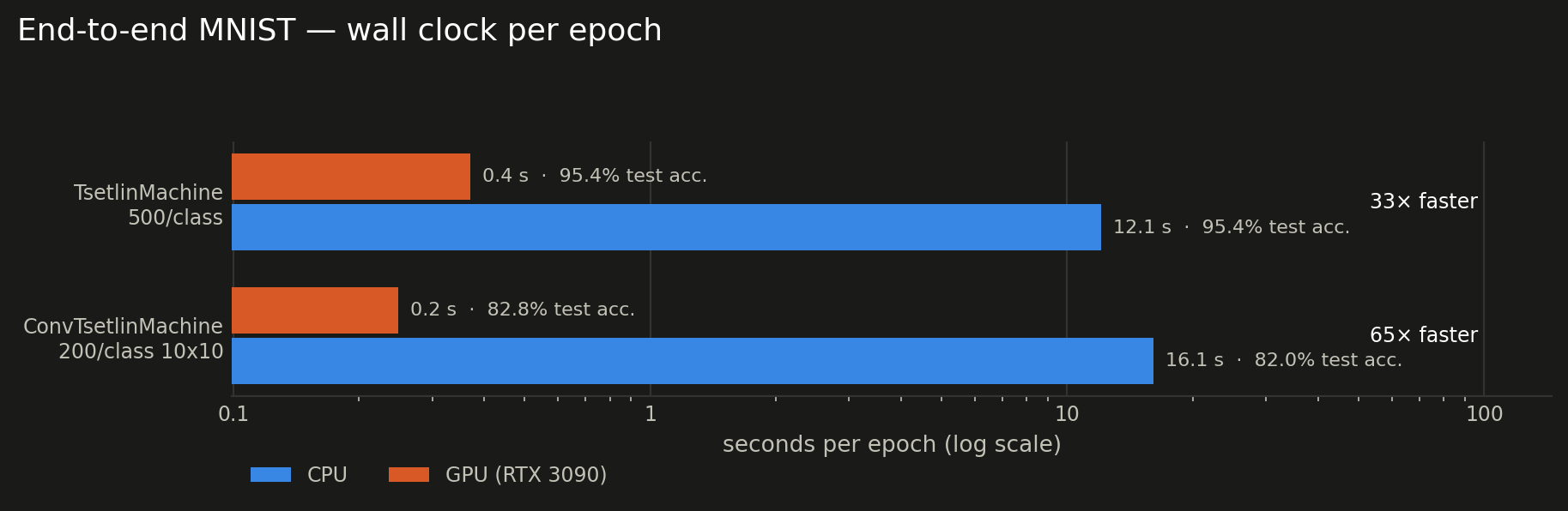
Synthetic micro-benchmarks flatter whichever device wins the micro-benchmark, so here is the whole thing end to end, Trainer.fit included:

• ConvTsetlinMachine 200/class 10x10 — 0.2 s/epoch on the GPU vs 16 s on the CPU (65×), 82.8% test accuracy
• TsetlinMachine 500/class — 0.4 s/epoch on the GPU vs 12 s on the CPU (33×), 95.4% test accuracy

Accuracy matches across devices to within run-to-run noise, as it should — only the wall clock moves. These are short runs at a modest clause budget; see Benchmarks for what longer runs reach.

End-to-end MNIST

model	device	train examples	epochs	s / epoch	examples/s	test accuracy	GPU peak memory
ConvTsetlinMachine 200/class 10x10	cpu	10,000	1	16.12	620	0.8200	—
ConvTsetlinMachine 200/class 10x10	cuda:0	10,000	1	0.25	40,266	0.8280	474 MB
TsetlinMachine 500/class	cpu	60,000	3	12.08	4,966	0.9541	—
TsetlinMachine 500/class	cuda:0	60,000	3	0.37	162,193	0.9541	236 MB

Reproducing

./benchmarks/run_benchmarks.sh                  # every suite, cpu + cuda:0
./benchmarks/run_benchmarks.sh --quick          # ~1 min smoke test
./benchmarks/run_benchmarks.sh -s batch models  # a subset
./benchmarks/run_benchmarks.sh --plots-only     # re-render from existing results

The raw records live in benchmarks/results/versions/0.6.0/cpu_vs_gpu.json (one folder per library version); benchmarks/plot_benchmarks.py turns them into the figures above and writes this page.