Why a Tsetlin machine learns what it learns

How a Tsetlin machine learns describes the algorithm. This page explains what it converges to, following Chapter 2 of Granmo's An Introduction to Tsetlin Machines. The argument is short. Every automaton is a random walk, so learning is a Markov chain, and its long-run behaviour can be computed exactly. Doing so shows why s acts as a frequency threshold, why more automaton states make the decisions sharper, and why the vote margin T keeps clauses from getting stuck in bad configurations.

Every number and figure on this page is computed exactly from the book's chains by scripts/make_concept_figures.py. --check prints them next to the values in the book, and they agree.

Scope

The analysis covers the classical algorithm: one example at a time, unweighted clauses, no clause budget. It also follows the book's convention that a True literal of a matching clause is always memorised (boost_true_positive=True, the library default). Batched feedback, clause weights and max_included_literals are outside it; see Batched vs sequential feedback for how far batching moves away from this picture.

One literal is a Markov chain

Look at a single literal L in a clause for class Y, and let the clause contain nothing else. Each training example is one of four kinds, and each kind moves the literal's automaton in a fixed way:

example	feedback	what happens to L
L true, class Y	Recognize (Type Ia)	one step towards memorized
L false, class Y	Recognize or Erase (Type Ia / Ib)	one step towards forgotten, probability 1/s
L false, other class	Reject (Type II)	one step towards memorized, only while forgotten
L true, other class	none	stays

The next position depends only on the current one and on the example drawn, so the position is a Markov chain. Its transition probabilities follow from how often each kind of example occurs: P(L | Y) P(Y), P(not L | Y) P(Y) and so on.

The chain of one literal with four memory positions. Reject feedback pushes a literal up only while it is forgotten, so it can add a literal to a clause but never makes it stick.

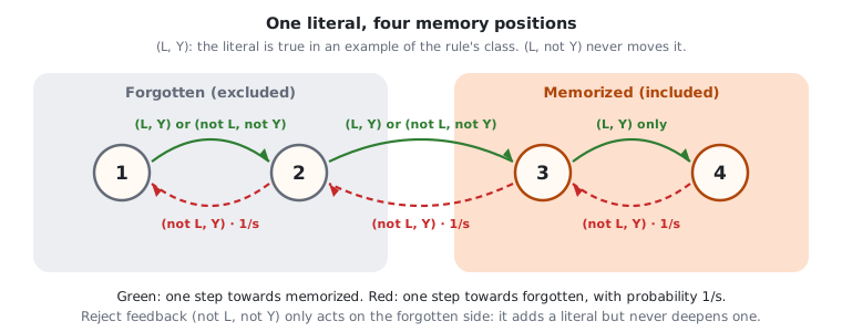
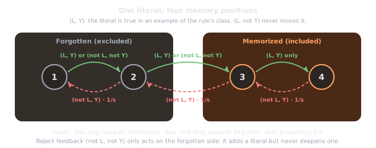
A Markov chain of this kind settles into a stationary distribution: the fraction of time it spends in each state in the long run. The distribution does not depend on where the chain started. For the literal it is the answer to "how likely is L to be part of the clause after learning?".

What the stationary distribution says

The book solves the four-state chain in closed form (its Table 2.1). Each state's probability is a product of factors, and each factor is one property of the learned clause:

• Frequent literals are memorised. The higher P(L | Y), the more mass sits on the memorized side.
• Infrequent literals are forgotten. The higher P(not L | Y), the more mass sits on the forgotten side.
• s moves the threshold. Forgetting happens with probability 1/s, so a larger s lets rarer literals survive. Roughly, a literal is kept when it is true in more than 1/s of the class's examples.
• Discriminative literals are preferred. A literal that is often true for Y and often false for the other classes gets pushed up by both Recognize and Reject feedback.
• Each extra memory state sharpens the decision exponentially. Every factor appears once per step away from the boundary. With more states the distribution piles up at the ends, and the literal is either clearly in or clearly out.

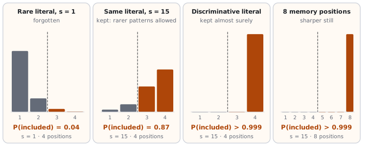
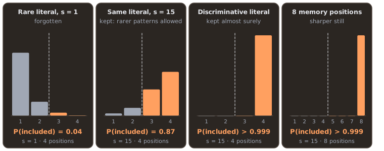
The book's four single-literal scenarios. A literal true in only 10 % of its class is dropped at s = 1 and kept at s = 15. A discriminative literal is kept almost surely, and doubling the memory concentrates the mass at the deepest position.

The four scenarios, in numbers:

scenario	share of class Y	L true within Y	L false within other classes	s	positions	P(included)
rare literal, carries no information	0.9	0.1	0.9	1	4	0.04
the same, slower forgetting	0.9	0.1	0.9	15	4	0.87
discriminative literal	0.82	0.99	0.5	15	4	> 0.999
the same, deeper memory	0.82	0.99	0.5	15	8	> 0.999

In the first two rows the literal is independent of the class. Whether it is kept depends only on whether it clears the 1/s frequency threshold.

Literals play a game

With two literals in one clause, each literal still moves on its own, but the feedback it receives depends on the other one, because the clause matches only if every included literal is true. The book frames this as a game in the style of the Prisoner's Dilemma. Each literal decides, without communicating, whether to be part of the clause, and the payoff depends on both decisions. The joint position of the two literals is again a Markov chain, now with 8 × 8 = 64 states for 8 memory positions each.

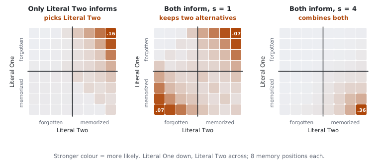
Where two literals settle. Left: only Literal Two predicts the class, and the clause keeps Literal Two alone. Middle: either literal predicts the class with precision 0.9, and at s = 1 the clause alternates between them. Right: the same data at s = 4, and the clause keeps both, reaching precision 0.99.

Four outcomes, from the book's Tables 2.5 to 2.8:

1. It selects informative literals. When only one literal carries information about the class, that one is memorised and the other is forgotten.
2. It keeps alternatives alive. When two literals are equally good on their own, the distribution has two peaks. During one long run the clause visits both.
3. It picks the best literal. When one literal is better than the other, the peak sits on the better one.
4. It combines literals for precision. Raising s allows rarer, more specific patterns. The pair L1 AND L2 is true less often but predicts the class with precision 0.99, and at s = 4 it becomes the most likely clause.

No literal ever sees the others. Coordination emerges from the three feedback types alone, which is why the learning rule is so short.

Clauses interact through the vote margin

The last step is several clauses. The book's example is Y = x1 OR x2 with 10 % label noise, learned by two clauses for Y. The only correct pair is one clause x1 and one clause x2. The clause x1 AND x2 is also correct whenever it fires, but it misses every example in which only one of the two literals is true.

Without a vote margin, every clause gets feedback on every example, so each clause learns independently and both converge to the same thing. Here that is x1 AND x2, a local optimum that fires on only one of the three input patterns for which Y holds.

With T = 2, a clause gets feedback with a probability that depends on how many clauses already vote. Once one clause covers an example, the other one is less likely to be trained on it, so the two clauses spread over different parts of the data.

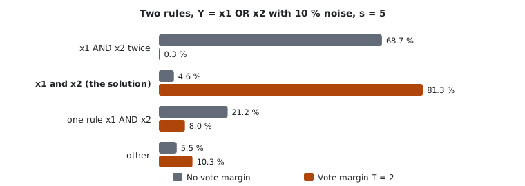
Two clauses learning x1 OR x2. Without a vote margin, both clauses become x1 AND x2 about two thirds of the time. With T = 2, that configuration almost disappears and the correct pair dominates.

pair of clauses after learning	no vote margin	T = 2
x1 AND x2 twice (local optimum)	68.7 %	0.3 %
x1 and x2 (the solution)	4.6 %	81.3 %

The book does not state s for this example. s = 5 reproduces its peak probabilities (0.31 without the margin and 0.16 with it, against 0.306 and 0.154 computed). The book describes the bad configuration as having zero probability with the margin; the exact chain gives it 0.3 %.

Learning never stops

All three results share one property. The outcome of learning is a probability distribution over clauses, not a single clause, and it does not depend on the initialisation. A Tsetlin machine keeps moving between the configurations that distribution favours. That has practical consequences:

• runs with different seeds end at different, equally good, rule sets;
• the clause set keeps changing late in training, so a single epoch's rules are a snapshot;
• the end of training is a valid starting point for further training on new data.

What to take away

result	parameter	practical reading
a literal is kept when it is true in more than about 1/s of the class	s	raise s for longer, more specific clauses; lower it if clauses memorise noise
more memory states sharpen every decision exponentially	n_states	deeper memory makes clauses more stable but slower to change their mind
combining literals only pays once rare patterns are allowed	s	precise multi-literal rules need a large enough s
the vote margin steers clauses away from shared local optima	T	raise T with the number of clauses so they keep covering different sub-patterns

See also Hyper-parameters.

References

• O.-C. Granmo, An Introduction to Tsetlin Machines, Chapter 2, tsetlinmachine.org.
• O.-C. Granmo, The Tsetlin Machine – A Game Theoretic Bandit Driven Approach to Optimal Pattern Recognition with Propositional Logic, arXiv:1804.01508 (2018).