Segmentation¶

Semantic segmentation asks for a label at every pixel. This page explains why a convolutional Tsetlin machine cannot produce one, what torchtsetlin does instead, and which of the available context mechanisms actually move the numbers.

Why a convolutional TM cannot segment¶

In a convolutional TM a clause is a filter that slides over the image, and the clause's output for the image is the disjunction over all patch positions (Granmo et al., 2019):

\[c_j \;=\; \bigvee_{b=1}^{B} c_j^{\,b}\]

That OR is exactly what gives a CTM its translation tolerance, and exactly what destroys a dense output: afterwards the model knows a pattern occurred somewhere, not where. In the code it is one line — matches.any(dim=1) at the end of _ConvMixin._evaluate. Every published TM aggregates patches this way, and CTM-UNet (Liu & Abeyrathna, ISTM 2025) is the only paper that works around it, by keeping the block output as a vote map.

If you want the unreduced tensor for a convolutional model — to plot where a clause fires, or to stack blocks — use model.patch_clause_outputs(x), which returns (B, Py, Px, C). It is an inspection tool: it does not make the model learn a dense output, because the feedback path still collapses the patch axis.

The dense head¶

SegmentationTsetlinMachine keeps the patch axis instead. Every pixel contributes one kh × kw neighbourhood of the Boolean planes, and that neighbourhood is an ordinary example of a flat Tsetlin machine whose label is the pixel's class:

(B, Z, H, W)  --unfold, pad--> (B·P, Z·kh·kw)  --> clause outputs (B·P, C) --> votes (B·P, K)
                                                                              --> (B, K, H, W)

Folding the patch axis into the batch axis is the whole trick: with B' = B·P the vote sums, the Type I / Type II selection, the feedback counting and functional.apply_feedback all apply unchanged. A dense segmenter is a convolutional TM with padding="same", stride=1, no OR-pooling and a per-patch label taken from the centre pixel.

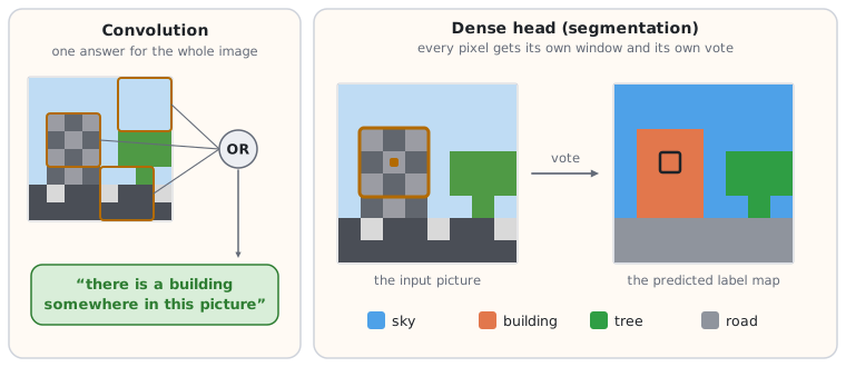
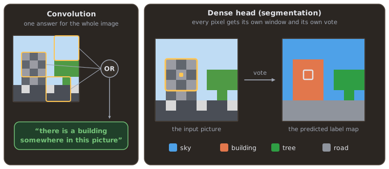
A convolutional machine ORing windows into one answer, next to a dense head painting a label per pixel — Left: the OR over windows gives one answer for the whole picture — it knows *that* there is a building, not *where*. Right: the dense head gives every pixel its own window and its own vote, and the votes form the label map.

This is CTM-UNet's CTM2D block without the disjunction, and the paper's K parallel machines are the K clause banks of one TsetlinMachine.

model = tt.SegmentationTsetlinMachine(
    n_classes=4, n_clauses=300, T=60, s=10.0, patch_size=3,
).to("cuda")
model.update(x, labels)        # x: (B, Z, H, W) Boolean, labels: (B, H, W) long
model.eval()
model.predict(x)               # (B, H, W) label map
model.vote_map(x)              # (B, K, H, W) per-pixel vote sums

forward() returns the folded votes (B·P, K), which is what keeps Trainer, metrics and interpret working unchanged; vote_map and predict are the segmentation-facing views.

Commit granularity is a real hyper-parameter¶

One batch of 8 images at 32×32 is 8 192 pixel-examples. Committing all of their feedback at once is a mini-batch of 8 192 — far past the point where batched feedback stops matching the classical algorithm (see Batched vs sequential feedback, which puts the onset at a couple of hundred on Noisy XOR). patches_per_commit bounds it.

Measured on make_segmentation_shapes (16×16, 3 classes, 100 clauses/class, 12 epochs, mean ± sd over 3 seeds):

`patches_per_commit`	pixel accuracy	mIoU	relative time
64	0.938 ± 0.001	0.741 ± 0.002	21×
128 (default)	0.940 ± 0.002	0.749 ± 0.009	11×
256	0.909 ± 0.019	0.659 ± 0.056	5.7×
512	0.898 ± 0.034	0.620 ± 0.097	3.0×
1024	0.886 ± 0.012	0.591 ± 0.029	1.7×
4096	0.814 ± 0.094	0.527 ± 0.073	1×

Two things to read off it. Quality is flat up to ~128 and then falls away; and the variance grows with the commit size, so a single large-commit run can look fine and the next one collapse. feedback_mode="sequential" is equivalent to patches_per_commit=1 — the exact classical algorithm, one pixel at a time, and correspondingly slow.

Context: what a `k × k` patch cannot know¶

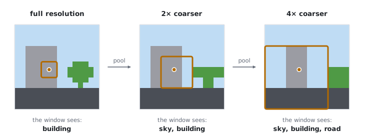
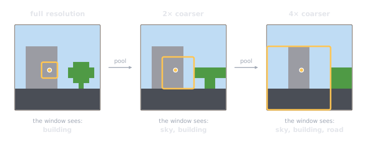
A 3×3 patch of building interior and a 3×3 patch of road look alike once illumination varies; separating them needs to know where the horizon is, which is information that does not exist inside the window. This is the gap an encoder–decoder closes in a CNN, and there are two TM-native ways to close it here.

Position literals (position_encoding=8) append thermometer-encoded patch coordinates, so a clause can say y > 12 AND NOT y > 18 — "only in these rows". Pass an integer to bound the feature count on large images; True uses one bit per row and column, which is fine at 32 px and ruinous at 512.

A multi-scale pyramid (data.PyramidEncoder) OR-pools the Boolean planes, takes the same k × k patch at each level and resamples every level back to full resolution, so a clause reads the pixel's neighbourhood and the coarse structure around it. Feed the result to a model with patch_size=1. No float parameter and no gradient anywhere — the pooling is functional.boolean_pool and the machinery to pass one machine's votes into another as ordered Boolean planes is functional.thermometer_cast.

The same 3 by 3 window on the full image and on 2x and 4x coarser copies, covering more and more of the scene — Why the pyramid helps. On the full image, a 3 × 3 window inside the building sees only wall; on coarser copies the same window reaches the sky and the road. (The encoder OR-pools Boolean planes; the colours here are for readability.)

Measured on make_scenes (32×32, 4 classes, 220 train / 80 test, 300 clauses/class, 8 epochs, 4-bit colour thermometer):

	pixel acc.	mIoU	sky	building	tree	road
row prior, no image content	0.876	0.410	0.715	0.000	0.000	0.923
single scale 3×3	0.934	0.798	0.980	0.505	0.808	0.898
pyramid 1×/2×/4×	0.967	0.874	0.982	0.699	0.867	0.950
single scale + position	0.991	0.946	0.998	0.894	0.903	0.989
pyramid + position	0.993	0.959	0.996	0.921	0.926	0.992

Building IoU is the column that matters: 0.505 with no context, 0.699 with the pyramid, 0.894 with position literals, 0.921 with both. Both mechanisms work and they compose.

Read mIoU, not pixel accuracy

The first row is a classifier that has never seen a pixel — it labels each pixel by the most common class in its row — and it already reaches 0.876 pixel accuracy, because these scenes have a stable vertical layout. It scores 0.410 mIoU, and zero on two of the four classes. Any dataset with a consistent layout has a floor like this; report it alongside your numbers. It is the same objection that applies to CTM-UNet's headline 96.35%, which is a binary sky-vs-background task.

A corollary for the model: position literals are so effective here partly because the layout is fixed. On data where the structure moves — cardiac MRI at varying slice positions, microscopy — expect them to help much less, and lean on the pyramid instead.

Class imbalance¶

Background dominates every real segmentation set, and a Tsetlin machine has no loss to reweight. The only lever is which pixels produce feedback, which is class_feedback_p: a per-class probability that a pixel takes part in an update. data.balanced_class_probabilities(labels, K, floor=0.05) computes the equalising choice.

It is a rescue, not a default. On the scenes above it lifts the pyramid-only run from 0.874 to 0.927 mIoU (building 0.699 → 0.842), and costs 0.05 mIoU once position literals are on, because by then the model can separate the classes anyway and throwing away 95% of the road pixels is pure loss. Reach for it when a specific class is being lost, and check the per-class IoU afterwards.

Cost¶

Dense evaluation is H·W clause evaluations per image — roughly 1000× a flat classifier on a 32×32 input. Measured on a 16-core CPU, 4 planes, 4 classes, 100 clauses/class, batch of 8 images: about 35 000 px/s training and 1 090 000 px/s predicting, so prediction is ~30× cheaper than learning. Above ~64 px, use a GPU. _chunk_elements_per_example scales the chunk size with P · (8C + 4F); if you override it, get it right or chunking collapses into many tiny chunks.

What not to build¶

CTM-UNet puts trainable Conv2D layers in front of each CTM block. No gradient can cross a Tsetlin machine, so by the paper's own account those layers are a frozen random projection; measured in examples/notebooks/05_ctm_unet_segmentation.ipynb they cost 5.5 points of pixel accuracy, because they mix the bit planes and the thresholding that follows discards the ordering the thermometer encoding was built to preserve. A clause can only refer to the bits it is handed. Use the Boolean pyramid instead.