Convolution

A convolutional Tsetlin machine (Granmo et al., 2019; book chapter 4) lets clauses look for patterns anywhere in an image, sequence or volume instead of memorising absolute pixel positions.

Why convolution

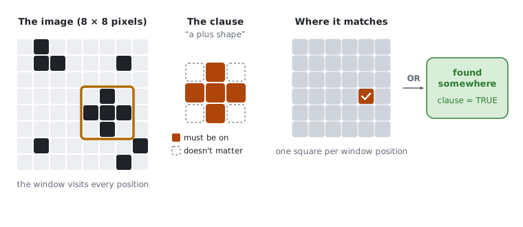
Take 4 × 4 black-and-white images of circles and crosses that can appear in any of the four corners (the book's example). A flat Tsetlin machine sees 16 pixel features, so the same circle in a different corner is a different pattern: it needs one clause per position, four for the circle and four for the cross. A convolutional machine looks at the image through a 3 × 3 window and uses the window's 9 pixels as features, so the features are the same wherever the window is. One clause per shape is enough, and it stays one clause when the image grows; a larger image only adds window positions.

Patches and position literals

An input image (Z, H, W) of Boolean planes is cut into every kh × kw window (with a stride). Each window becomes a patch with

• Z * kh * kw pixel features, followed by
• thermometer-encoded coordinates: P_y - 1 bits [y > k] and P_x - 1 bits [x > k], where P_y, P_x are the number of window positions along each axis (position_encoding=True).

A clause that includes y > 2 AND NOT y > 5 therefore only matches windows in rows 3–5, i.e. it can learn where a pattern is allowed to appear — or ignore position entirely.

Position matters when the same local pattern means different things in different places. The book's example is a horizontal stroke: at the top of a digit it is the bar of a 7, at the bottom it is the base of a 2. A clause that restricts the stroke to the upper rows stops matching the 2. Thermometer bits are used because two of them express a range, so a clause can describe a rectangular region with at most four position literals.

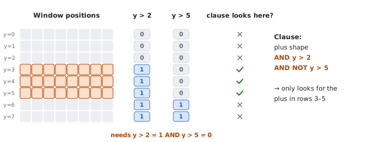
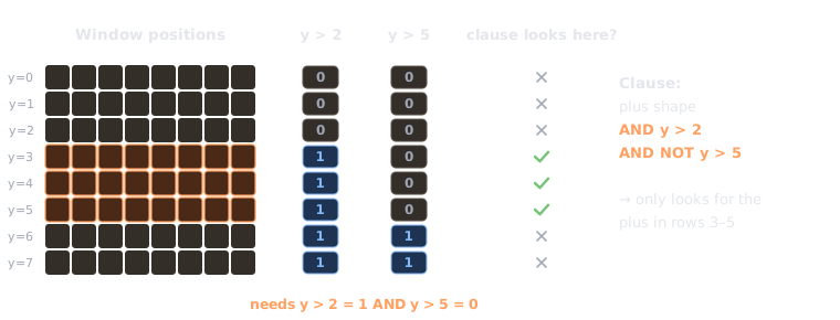
Position literals are thermometer bits too. Including y > 2 and NOT y > 5 restricts the clause to window rows 3–5; including none of them lets it match anywhere.

Evaluation and learning

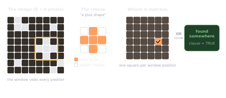
A clause is True for an image if it matches at least one patch (OR over patches). Vote sums, T and the Type I / Type II selection are unchanged. When a matching clause receives Type Ia or Type II feedback, one matching patch is drawn uniformly at random and its literals are used for the update; Type Ib (no match) needs no patch.

For a clause selected for feedback, the four cases are:

	clause matches some patch	clause matches no patch
example of the clause's class	Type Ia (Recognize) on one random matching patch	Type Ib (Erase), no patch needed
example of another class	Type II (Reject) on one random matching patch	no feedback

Different clauses end up specialising on different parts of an image: one on a wheel, one on the ground below it, one on a window. The image's class is decided by their summed votes. This cooperation is what T buys. With the book's T = 2 from Chapter 1, two matching clauses already satisfy the margin, so few clauses ever learn about a class. A larger T keeps feedback flowing until many clauses agree, so more of them learn to recognise different parts. That is why convolutional models use a much larger T relative to their clause count than flat ones (see Hyper-parameters).

A 3 × 3 clause is checked at every window position; the OR over positions makes it true for the image if it matches anywhere. That is why one clause can find a shape no matter where it appears.

torchtsetlin implements this with torch.nn.functional.unfold for the patches, a single matmul for all (patch, clause) matches and a gather of the randomly chosen patch rows for the feedback counts. The draw happens in _feedback_counts, over the selected feedback events only, so prediction costs one matmul and an OR — no randomness at all — and each event draws its own patch (a coalesced clause can take Type Ia and Type II in the same update). Memory is bounded by chunking the batch (see Batched vs sequential feedback).

model = tt.ConvTsetlinMachine(
    n_classes=10, n_clauses=200, T=100, s=10, patch_size=10, weighted=True,
).to("cuda")
model.update(images, labels)          # images: (B, 1, 28, 28) Boolean
model.clause_patch(0)                 # (Z, kh, kw) map: 1 = must be on, -1 = off, 0 = free
model.clause_region(0)                # allowed window rows/columns of clause 0
tt.viz.plot_conv_clauses(model, range(16))

Variants: ConvCoalescedTsetlinMachine (shared clauses, multi-label capable), ConvRegressionTsetlinMachine, Conv1dTsetlinMachine for sequences (B, Z, L), and the 3D models below for volumes (B, Z, D, H, W).

3D volumes

Nothing in the algorithm above depends on the patches coming from a 2D grid. Evaluation is an OR over a set of patches, and feedback draws one matching patch from that set. A 3D machine changes only how the set is built:

• the window is kd × kh × kw and slides along depth, rows and columns, giving P = Pd · Ph · Pw positions, with P_a = ⌊(N_a − k_a) / s_a⌋ + 1 per axis;
• each patch has Z · kd · kh · kw voxel features;
• position literals use three thermometers, d > k, y > k and x > k. A clause's position literals therefore describe an axis-aligned box of window positions, and clause_region returns it as {"d": …, "y": …, "x": …}.

The window covers three consecutive slices and visits every position along x, y and depth. There is one match map per depth offset, and the OR over all of them is the clause output.

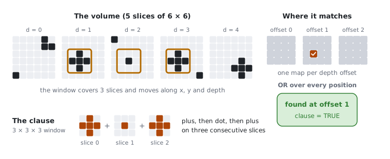
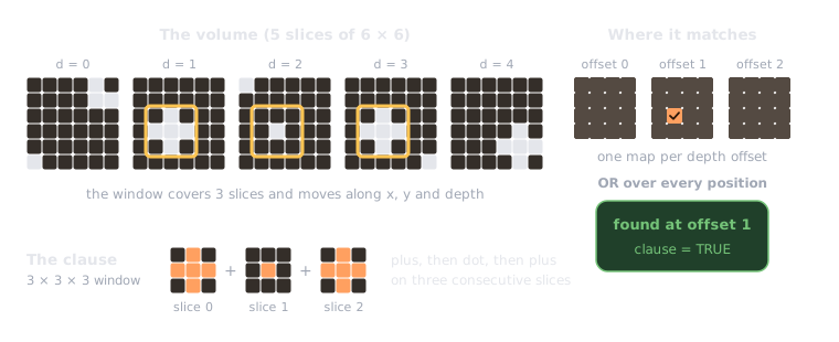
Conv3dTsetlinMachine reuses the 2D clause evaluation and feedback code unchanged, because that code only ever sees a (B, P, 2F) tensor of patch literals. A consequence that the tests pin: with D = kd = 1, the 3D model builds bit-for-bit the literals of ConvTsetlinMachine and, under the same seed, trains to the same automata.

Why not just stack the slices as channels? That works, and it equals a 3D machine whose window spans the whole depth (kd = D). But such a window cannot slide along depth, so a pattern that can occur at any depth needs one clause per depth offset. A window with kd < D covers all offsets with a single clause. For the concept "some voxel is on" in a depth-D column, the stacked model provably needs at least D clauses, while the 3D model needs one.

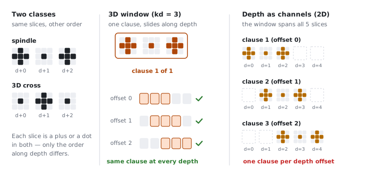
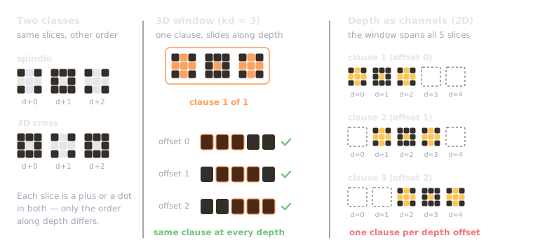
The two classes of make_3d_shapes use the same slices in a different order. A kd = 3 window learns the order once and slides it through depth; a 2D model on stacked slices sees all five at once and has to learn each depth offset as a separate clause.

model = tt.Conv3dTsetlinMachine(
    n_classes=2, n_clauses=20, T=15, s=10, patch_size=3, position_encoding=False,
)
model.update(volumes, labels)         # volumes: (B, Z, D, H, W) Boolean
model.clause_patch(0)                 # (Z, kd, kh, kw): 1 = on, -1 = off, 0 = free
model.clause_region(0)                # {"d": (lo, hi), "y": ..., "x": ...}
model.patch_clause_outputs(volumes)   # (B, Pd, Ph, Pw, C) match maps
tt.viz.plot_conv_clauses(model, range(8))   # each clause drawn slice by slice

Conv3dCoalescedTsetlinMachine and Conv3dRegressionTsetlinMachine are the 3D versions of the coalesced and regression variants. Use it for MRI or CT stacks (slices, H, W), or put time on the depth axis for cine sequences (frames, H, W).

Memory. The cost scales with P, and volumes have many positions: a 12 × 64 × 64 stack with a 3 × 7 × 7 window has 33 640. When one volume would exceed max_chunk_elements, which happens with many clauses, the model splits the patch axis into blocks. This is exact: the OR over patches is the OR of the per-block ORs, and the random matching patch is the best of the per-block winners, so the draw has the same distribution. Set patches_per_chunk to choose the block size yourself. An in-plane stride such as stride=(1, 2, 2) is the cheaper lever, since it cuts P four-fold. Measured numbers are in CPU vs GPU.

Runnable examples

Walked through in Convolution on generated data and MNIST:

script	model	what it demonstrates
examples/shapes_conv.py	ConvTsetlinMachine	one clause beats a flat machine that has to memorise every position (1.000 on every seed, against 0.55–0.91), and what position_encoding costs on a translation-invariant task
examples/conv1d_ramps.py	Conv1dTsetlinMachine	a motif anywhere in a thermometer-encoded signal; the clauses print as the ramp they detect
examples/conv_regression_blobs.py	ConvRegressionTsetlinMachine	reading a continuous quantity (a square's side length) off an image
examples/shapes_conv3d.py	Conv3dTsetlinMachine	shapes that differ only in their slice order: the 3D model scores 1.000 on every seed, stacking slices as channels 0.83–0.98, a flat TM 0.73–0.80
examples/mnist_conv.py	ConvTsetlinMachine, ConvCoalescedTsetlinMachine	the real thing: 10×10 windows, adaptive thresholding, --stride, --coalesced

Tips

• Booleanize images with AdaptiveThresholdEncoder (MNIST-like) or ColorThermometerEncoder (RGB) — see Booleanization.
• Typical MNIST settings from the literature: 10 × 10 windows, 2000–8000 clauses per class, T around 1.25–12.5 × clauses-per-class, s 5–10, weighted clauses.
• Set position_encoding=False for tasks that are fully translation invariant; position literals otherwise make clauses more specific and slower to generalise on small data. This holds in 3D too: on make_3d_shapes, accuracy drops from 1.000 to 0.48 with them on.